Page 82 - BKT Annual Report 2024 EN
P. 82
Notes to the Consolidated Financial Statements for the year ended 31 December 2024                                                                          Notes to the Consolidated Financial Statements for the year ended 31 December 2024
         (amounts in USD, unless otherwise stated)                                                                                                                                                               (amounts in USD, unless otherwise stated)


         (a) Introduction and overview
         The Bank has exposure to the following risks from financial instruments:                                                Financial Instruments             31 December 2024                        31 December 2023
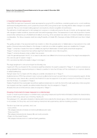
                                                                                                                                 Credit Risk
         •  credit risk
         •  liquidity risk                                                                                                                                  Exposure                                Exposure
                                                                                                                                                                                                                           Net exposure
         •  market risks                                                                                                                                       before   Impairment  Net exposure       before   Impairment  for credit risk
                                                                                                                                                                                   for credit risk
         •  operational risks                                                                                                                              impairment                              impairment

         This note presents information about the Bank’s exposure to each of the above risks, the Bank’s objectives, policies and processes   A. Credit risk exposure relating to balance sheet items
         for measuring and managing risk, and the Bank’s management of capital.                                                  Cash and Balances with
         A financial instrument is any contract that gives rise to the right to receive cash or another financial asset from another party (financial   Central Bank   677,670,397   -   677,670,397   676,805,203      -   676,805,203
         asset) or the obligation to deliver cash or another financial asset to another party (financial liability).             Placements and Balances
         Financial instruments result in certain risks to the Bank. The most significant risks facing the Bank are credit risk, liquidity risk and market   with banks   337,792,699    (15,598)   337,777,101   342,476,395  (14,075)  342,462,320
         risk. Market risk includes foreign currency risk, interest rate risk and other price risks.
                                                                                                                                 Investment securities -    37,964,615          -     37,964,615   11,759,570           -    11,759,570
                                                                                                                                 measured at FVTPL
         Risk management framework                                                                                               Investment securities -
         The Board of Directors has overall responsibility for the establishment and oversight of the Bank’s risk management framework. The   measured at FVOCI   1,364,977,373   -  1,364,977,373   1,103,640,557      -  1,103,640,557
         Board has established the Bank Risk Committee, Asset and Liability Committee (ALCO), Investment Committee, Risk Management   Investment securities -
         Group and Credit Committees, which are responsible for developing and monitoring Bank risk management policies in their specified   measured at amortised cost   2,261,652,165    (9,344,022)  2,252,308,143   2,320,318,180  (19,470,943)  2,300,847,237
         areas. All these bodies report regularly to the Board of Directors on their activities.
                                                                                                                                 Loans to banks            139,349,673    (537,627)   138,812,046   136,349,523  (1,518,985)  134,830,538

         The Bank’s risk management policies are established to identify and analyse the risks faced by the Bank, to set appropriate risk limits and
         controls, and to monitor risks and adherence to limits. Risk management policies and systems are reviewed regularly to reflect changes   Loans to customers   1,959,808,659    (50,762,177)  1,909,046,482   1,748,606,735  (54,577,751)  1,694,028,984
         in market conditions, products and services offered. The Bank, through its training and management standards and procedures, aims
         to develop a disciplined and constructive control environment, in which all employees understand their roles and obligations.  Other assets        13,868,224    (365,259)   13,502,965   10,598,516    (896,549)    9,701,967

                                                                                                                                 Total Assets             6,793,083,805    (61,024,683)   6,732,059,122   6,350,554,679    (76,478,303)  6,274,076,376
         The Bank Audit Committee is responsible for monitoring compliance with the Bank’s risk management policies and procedures, and
         for reviewing the adequacy of the risk management framework in relation to the risks faced by the Bank. The Bank Audit Committee is   Off balance sheet items
         assisted in these functions by Internal Audit. Internal Audit undertakes both regular and ad-hoc reviews of risk management controls
         and procedures, the results of which are reported to the Audit Committee.                                               Undrawn credit
                                                                                                                                 commitments               272,805,545          -    272,805,545   290,078,945          -   290,078,945
         (b) Credit Risk                                                                                                         Outstanding cheques of       307,628           -       307,628       326,566           -       326,566
         Credit risk is the risk of financial loss to the Bank if a customer or counterparty to a financial instrument fails to meet its contractual   non-resident banks
         obligations, and arises principally from the Bank’s Loans to customers and other banks and investment securities. For risk management   Spot foreign currency    94,943,828   -   94,943,828   128,493,054     -   128,493,054
         reporting purposes, the Bank considers all elements of credit risk exposure (such as individual obligor default risk, country and sector   contract
         risk). The Bank has formed a Credit Committee to oversee the approval of requests for credits. Credit requests with amounts over EUR   Collaterals for loan portfolio   5,193,270,708   -   5,193,270,708   4,654,093,419  -  4,654,093,419
         2,000,000 are approved only upon decision of the Board of Directors of the Bank. There is a continuous focus on the quality of credits
         extended both at the time of approval and throughout lifetimes.                                                         Securities pledged as     227,990,707          -    227,990,707   145,749,308          -   145,749,308
                                                                                                                                 collateral
         Each business unit is required to comply with Bank credit policies and procedures. Regular audits of business units and Bank Credit   Interest rate swaps   98,920,539   -   98,920,539   103,994,039          -   103,994,039
         Risk Management Department processes are undertaken by Internal Audit.
                                                                                                                                 Total off balance sheet    5,888,238,955       -   5,888,238,955   5,322,735,331       -  5,322,735,331
         i. Maximum credit exposure
         The gross carrying amount of financial assets below also represents the Group’s maximum exposure to credit risk on these assets.   Total credit risk exposure    12,681,322,760    (61,024,683) 12,620,298,077   11,673,290,010  (76,478,303)  11,596,811,707
         Maximum exposures to credit risk before collateral and other credit enhancements as at 31 December 2024 and 31 December 2023
         are as follows:


        25                                                                                BANKA KOMBËTARE TREGTARE

